Units are log points, not percent. At this
magnitude the approximation is close (+3.5 log points ≈
+3.6%), but the exact transform is
exp(β) − 1.
The result
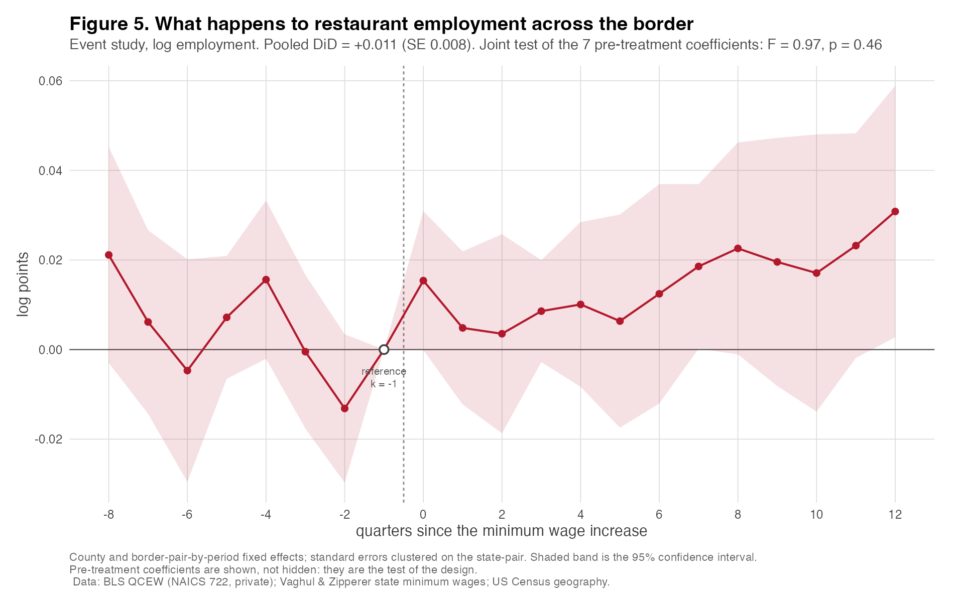
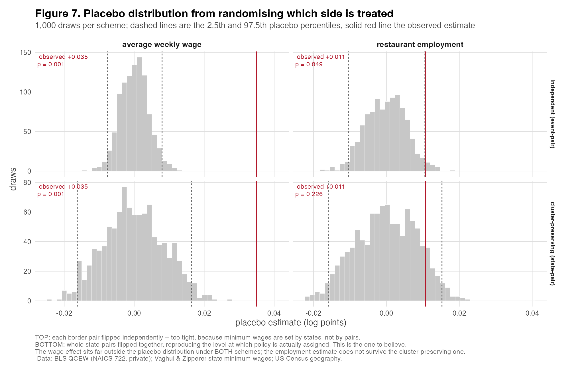
This is a bounded null, not evidence that minimum wages raise employment. The point estimate is positive but statistically insignificant, and under a randomisation test conducted at the level where policy is actually assigned it is indistinguishable from noise (p = 0.226).
What the interval does exclude is the conventional disemployment range: elasticities more negative than -0.04 lie outside it, ruling out the −0.1 to −0.3 band at this sample’s moderate increases (median differential $0.75). It is not proof of exactly zero.
The border design
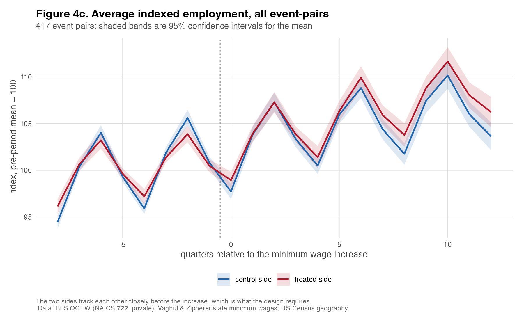
The counterfactual for a treated border county is its neighbour across the line. The preferred specification adds a border-pair-by-period fixed effect, so only the within-pair, within-quarter contrast identifies the effect and any shock common to the local economy is differenced out.
Treatment is a material increase in a state’s effective minimum wage
(max(state statute, federal)): at least $0.25 and at least 2.0%. Two
thresholds, because either alone admits the wrong events — a dollar rule treats $0.25 off
$7.25 like $0.25 off $13.00, and a percentage rule admits trivial CPI indexation.
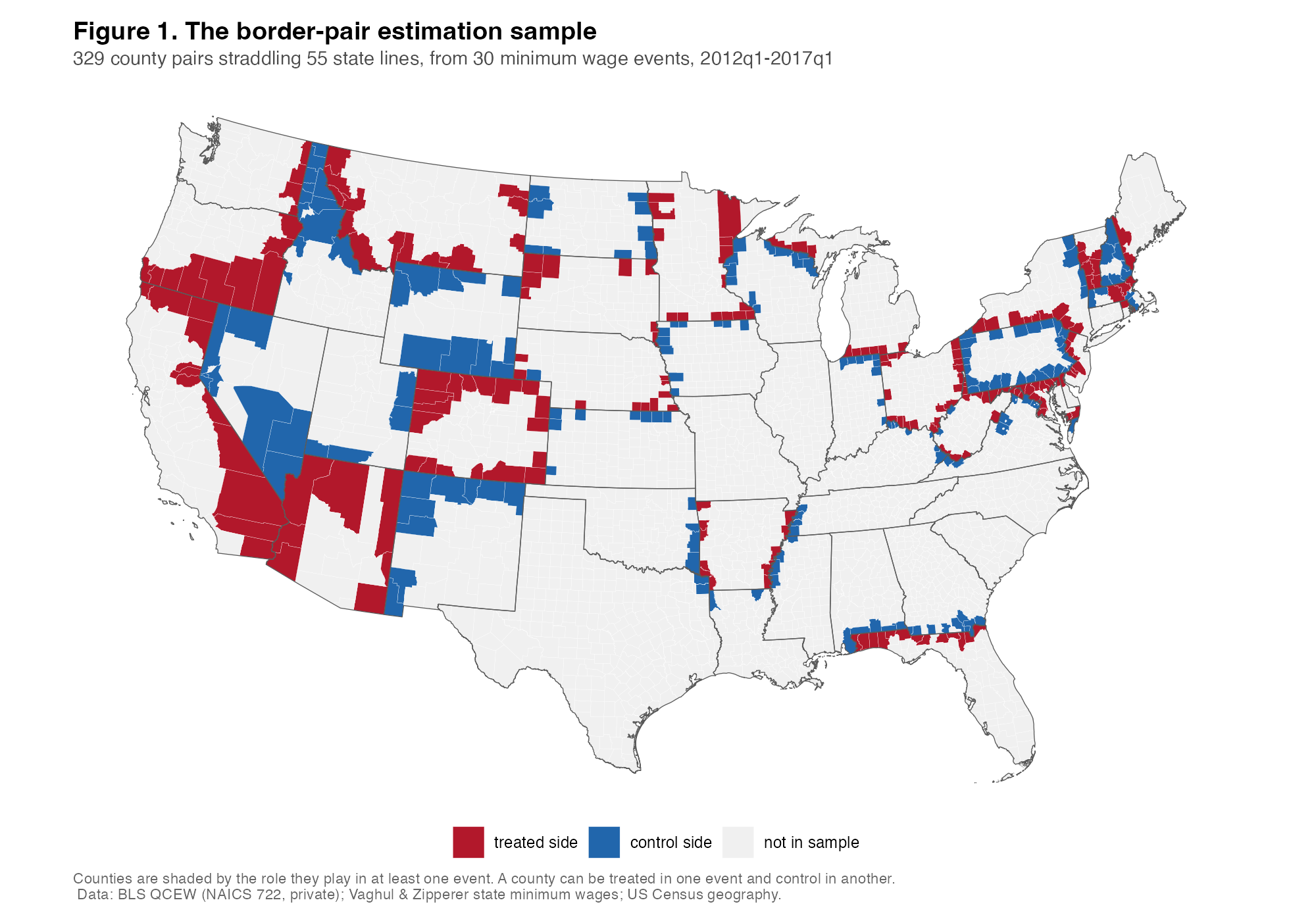
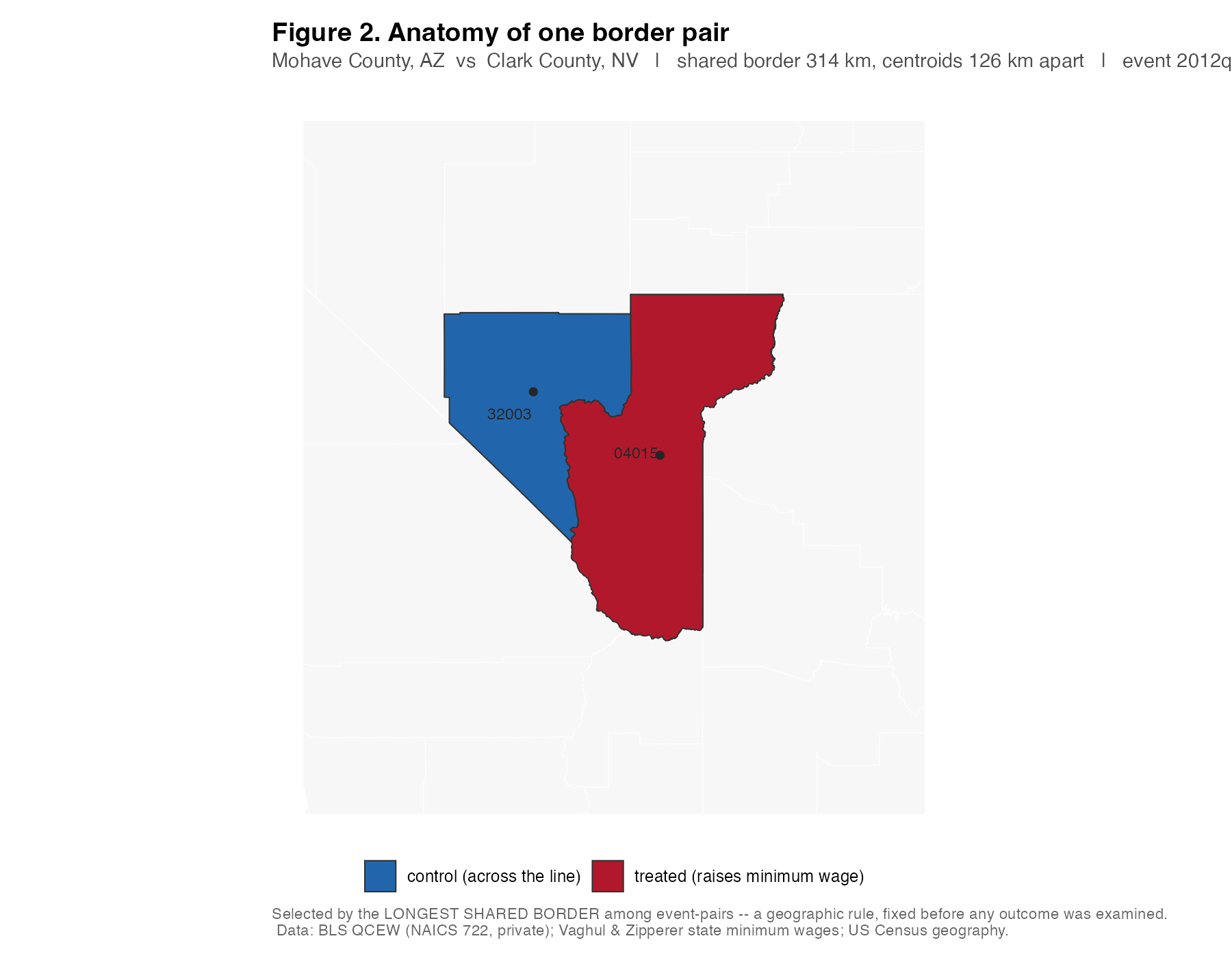
The Census adjacency file yields 2,616 directed cross-state links — exactly twice the 1,308
unordered pairs, a symmetry verified as a test rather than assumed. Shared border lengths are
computed from Census geometry in sf. This matters: 57 of the 1,308
“adjacent” pairs share no measurable frontier at all. They meet only at a
corner, and there is no border for a worker or a diner to cross.
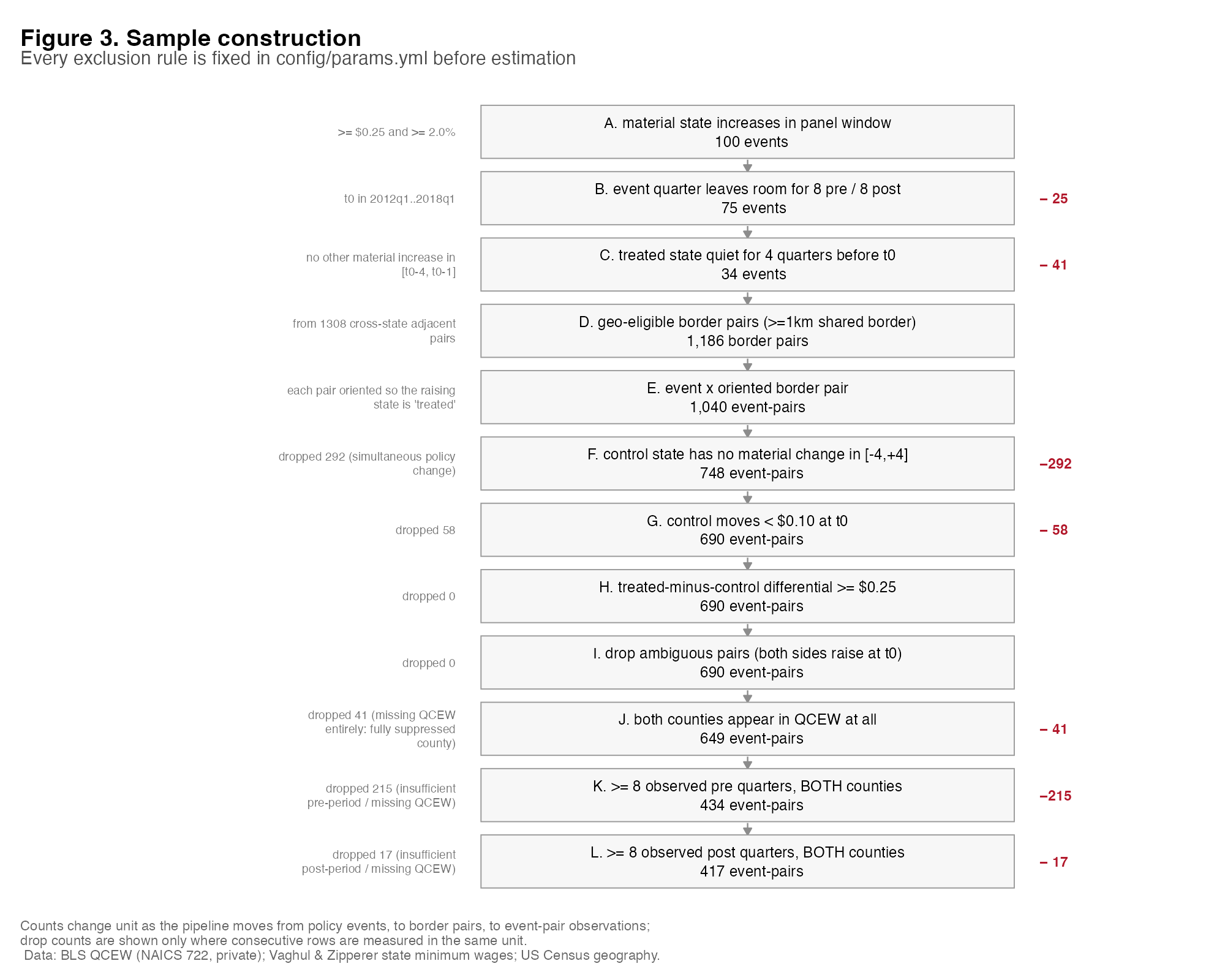
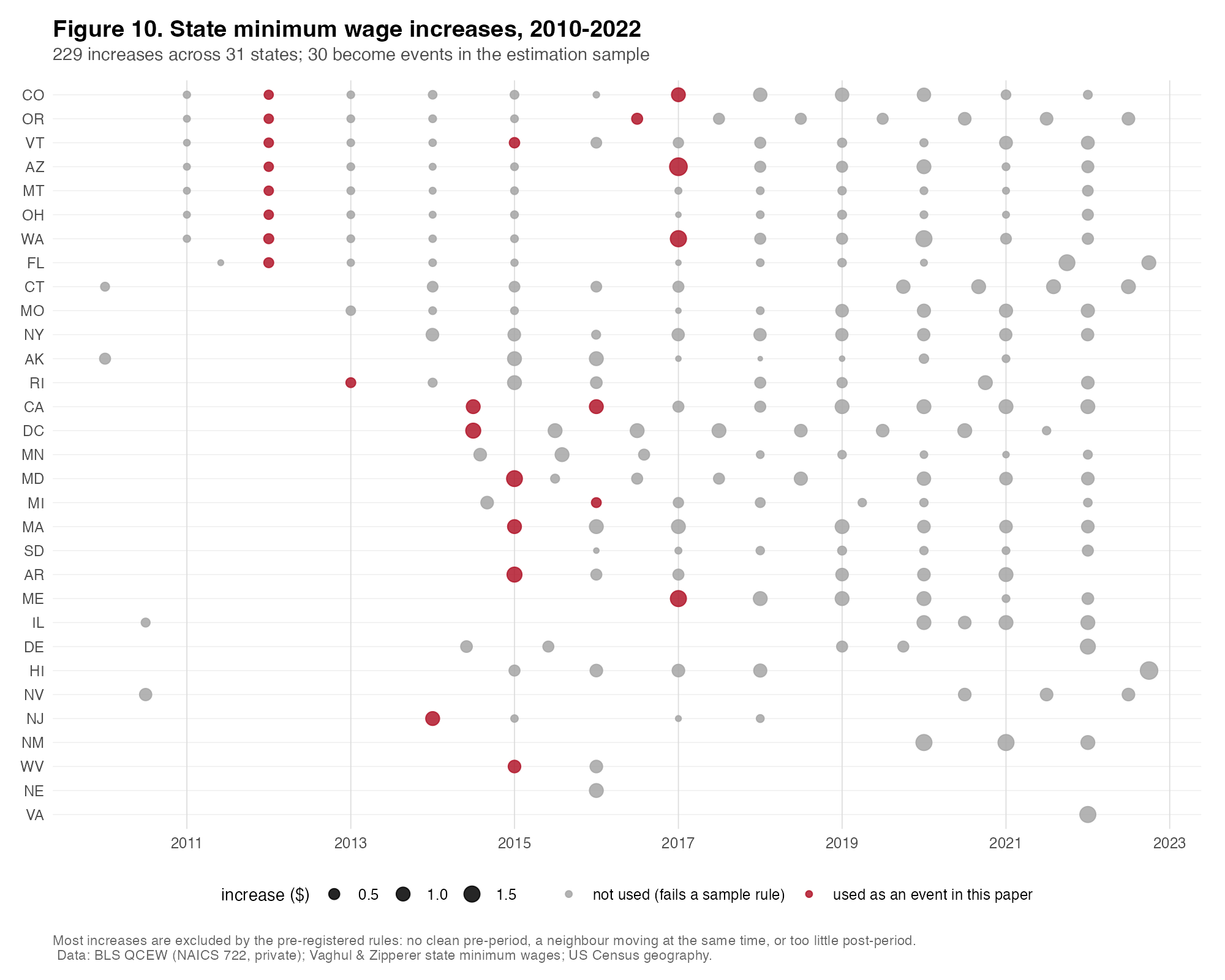
config/params.yml before estimation. The
single largest exclusion drops 292 candidate event-pairs because the control state also
moved materially within four quarters.Why inference matters
The sharpest methodological result here is that the randomisation scheme decides the answer. Keeping every pair, date and outcome fixed and randomising only which side of the border is called treated:
Minimum wages are legislated by states, not by county pairs, so the dependence structure of the randomisation has to match the dependence structure of policy assignment. The validation is that the cluster-preserving placebo standard deviation, 0.0084, almost exactly reproduces the clustered standard error, 0.0081 — the design-based and model-based approaches agree once the design-based one is done at the right level.
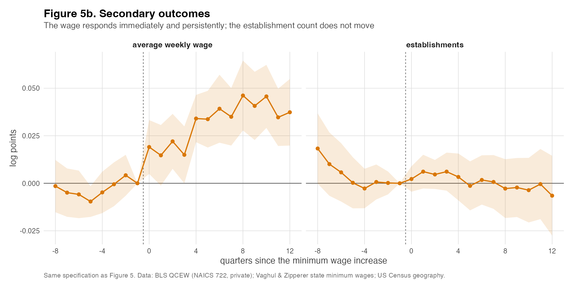
The wage effect clears both schemes at p = 0.001.
feols to
1.5e-15.Spillovers
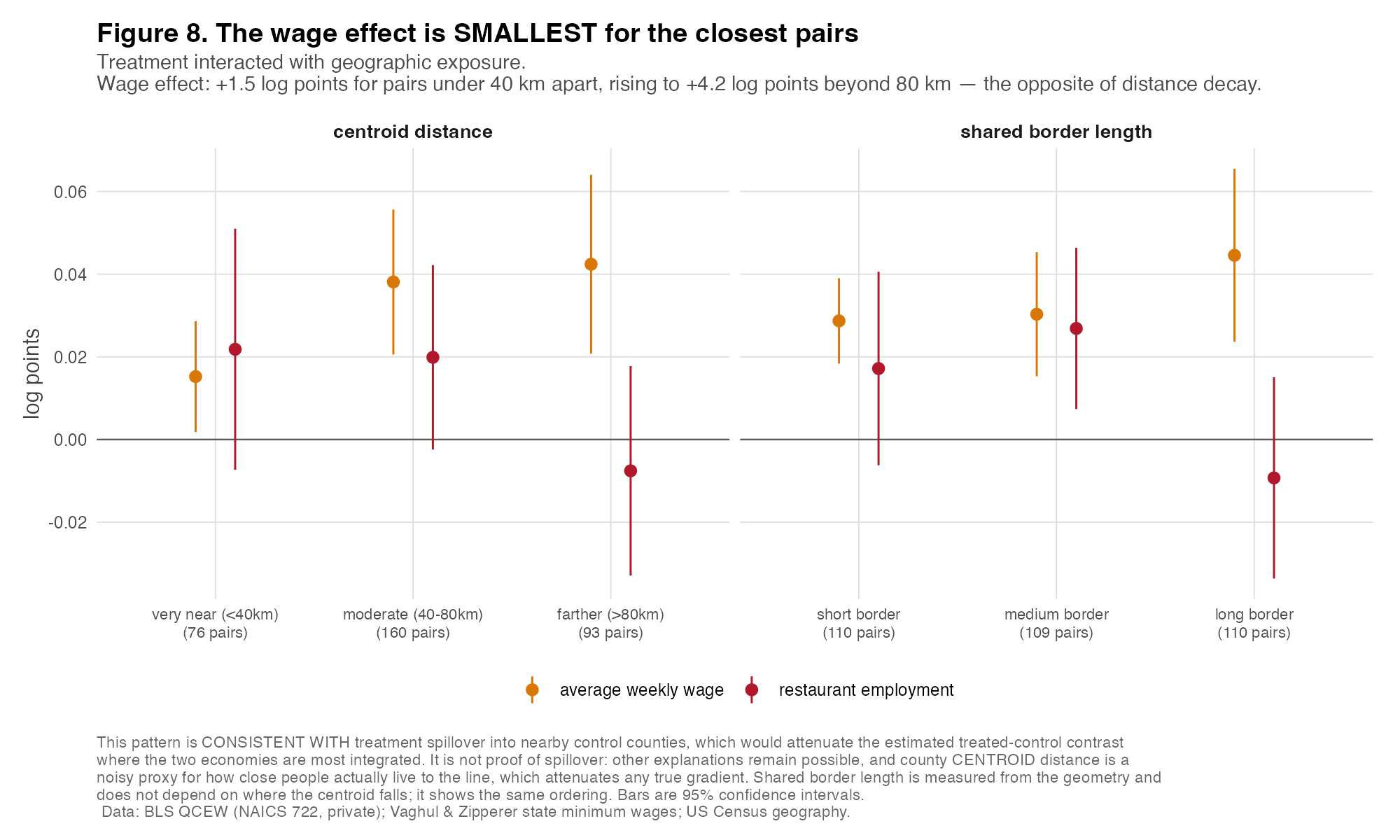
The wage effect is smallest for the geographically closest pairs: +1.5 log points under 40 km, rising to +4.2 log points beyond 80 km. The same ordering appears using shared border length, which is measured from geometry and does not depend on where a centroid falls.
This is the opposite of a simple “effect decays with distance” story. If the distance pattern reflects control-county spillovers — workers commuting across the line, forcing control-side restaurants to raise pay — then the main contrast would be biased toward zero. Other explanations remain possible, and county centroid distance is a noisy proxy for how close people actually live to the line. This is not proof of spillover.
Four estimators
Under staggered treatment, estimator disagreement is informative rather than noise to be averaged away. These are not averaged into a consensus number.
| Estimator | Log employment | Log weekly wage | |
|---|---|---|---|
| naive TWFE (pooled) | -0.019 | +0.047 | — |
| Callaway–Sant'Anna | -0.008 | +0.031 | — |
| Sun–Abraham | -0.006 | +0.034 | — |
| stacked border design primary | +0.011 | +0.035 | — |
The Goodman–Bacon decomposition shows why the naive TWFE figure is the outlier:
| 2×2 comparison | Weight | Avg. estimate | Control group |
|---|---|---|---|
| treated vs untreated | 0.760 | -0.015 | clean (control untreated) |
| later vs earlier treated | 0.154 | -0.018 | already treated — contaminated |
| earlier vs later treated | 0.086 | +0.010 | clean (control untreated) |
15.4% of the pooled TWFE weight sits on the contaminated block, where a later-treated county is compared against an already-treated one, so the control trend carries the earlier county’s own treatment dynamics. That block also has the most negative average estimate of the three — the mechanism dragging the pooled coefficient down. The three estimators built to avoid that contamination all land near zero.
A falsification that failed
Pre-trend joint test: F = 2.39, p = 0.033 (rejects). Six-quarter fake-date placebo: -0.013, p = 0.020 (significant).
Parallel trends is not credible for this outcome, so establishment estimates are reported descriptively and are not interpreted causally anywhere in the project. This is not buried: it demonstrates that the identification diagnostics have consequences.
Matching
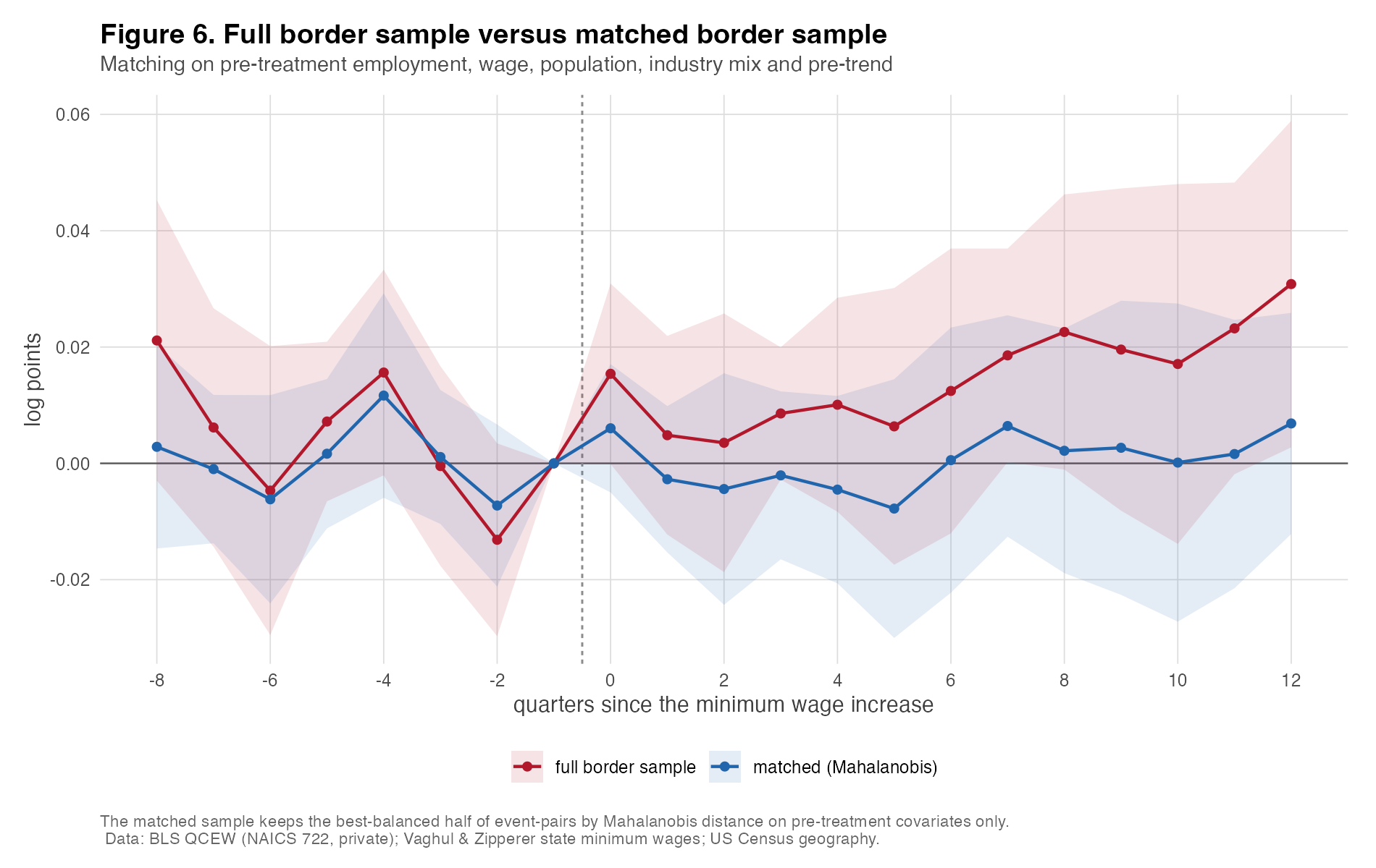
The strict pre-specified 0.5 SD caliper on every one of five covariates retained only 18 pairs — unacceptable power loss. That was discovered from sample size and covariate balance alone, before any treatment effect was computed, and the design was then revised using pre-treatment balance only: the best-balanced half by Mahalanobis distance, 209 pairs. The chronology is not rewritten; both samples are reported.
Matching variables are measured strictly at k < 0, enforced in code and independently verified by recomputing every stored covariate from pre-period data alone.
Data engineering
- BLS QCEW, NAICS 722 for outcomes and NAICS 10 to build the restaurant share of county employment used in matching.
- The convenient API only covers 2014 onward. For 2010–2013 the data sits in annual archives of roughly 470 MB each, from which one NAICS member is needed. The loader issues HTTP range requests to read the ZIP central directory and pull only the ~5 MB member required.
- Automated seam check in every build, because the source changes between 2013q4 and 2014q1: national restaurant employment grows +3.6% year-over-year across the seam, a normal rate, and the build fails above 10%.
- Suppression. QCEW withholds cells that would disclose an individual employer; they arrive as literal zeros with a disclosure flag. Read as zeros they would manufacture enormous fake swings, so they are set to missing (18.3% of county-quarters).
- Provenance. 88 source files with a SHA-256 manifest recording URL, timestamp, byte count and hash. Raw archives are not versioned — reproducibility comes from the download scripts plus hashes.
- Policy edge cases. 230 in-window changes with a federal-binding flag, faithful to the source including Colorado’s genuine CPI-indexed nominal decrease ($7.28 → $7.24).
Heterogeneity, marked exploratory
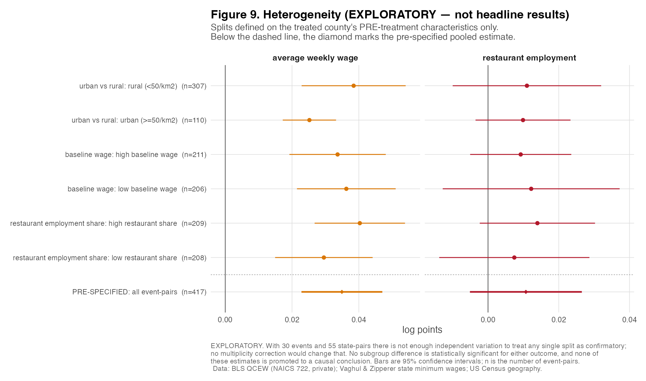
Three theory-driven splits on the treated county’s pre-treatment characteristics. The wage effect is present in every subgroup; the employment effect is null in every subgroup; and no subgroup difference is statistically significant for either outcome.
With 30 events and 55 state-pairs there is not enough independent variation to treat any single split as confirmatory, and no multiplicity correction would change that. These are reported so the whole picture is visible; none is promoted to a causal conclusion.
Limitations
- Parallel trends is an identifying assumption, not something the data can prove.
- Border counties can still differ from each other in unobserved ways.
- Minimum-wage increases may coincide with other state policy changes; the border-pair fixed effect removes what is common to the local economy but nothing state-specific.
- Cross-border spillovers may contaminate the controls.
- Treatment timing is staggered, which is why four estimators are compared.
- The establishment outcome fails pre-trend diagnostics.
- Matching cannot remove unobserved confounding.
- The 2019q4 endpoint intentionally excludes the pandemic period, reducing contamination from shocks correlated with the same state characteristics that predict minimum-wage increases. It does not remove all confounding.
- Results concern restaurant-sector county outcomes in this sample — border counties, moderate increases — not the economy at large.
- The null employment estimate is not proof of exactly zero effect.
Clustering choice moves the employment standard error only between 0.0071 and 0.0106 across six specifications, so no conclusion turns on it.
Reproduce
git clone https://github.com/Gariyuuu/copycat-economy.git
cd copycat-economy

python3 -m venv .venv
source .venv/bin/activate
pip install -r requirements.txt

./run_all.sh              # download, build, estimate, draw, test
./.venv/bin/python -m pytest tests -q   # 53 passed
Every analysis threshold lives only in config/params.yml, so there is exactly one
place a researcher degree of freedom can be exercised and it is version-controlled. Sample
construction never reads an outcome value — only whether a cell is observed.